
Two front monochromatic camera/laser systems provided stereo viewing and ranging, while the rear mounted camera was discriminant in the red, green, and IR spectral bandwidths to produce color images. Whereas the Imager for Mars Pathfinder (IMP) camera viewed the Martian scenes from a fixed platform at spatial resolutions that diminished with distance, the mobile rover was able to drive up to landforms, including those hidden from the IMP, to image them at higher resolution.
The rover cameras were built by the Microrover Flight Experiment Team at the Jet Propulsion Laboratory.
Primary objectives for the rover were 1) exit the lander as early as practical on the basis of lander stereoscopic images, 2) send initial vehicle performance and technology experiment data to the lander, 3) move a few meters and repeat objective #2, 4) acquire and transmit images showing the condition of the lander, 5) acquire images at the end of daily traverses for navigation purposes, or encounter, acquire, and transmit an image of a rock or soil patch for subsequent APXS analysis, 6) deploy APXS on the imaged rock or soil patch, if possible, for 1 to 10 hours duration for chemical analysis, 7) query the APXS for final data and transmit interim and final data to the lander, and 8) traverse diverse terrains and repeat objective #2.
An Extended Mission of 30 sols was planned and more than realized, as the governing spacecraft, rover and site-related factors permitted rover activities to continue for 81 sols. Extended Mission objectives were similar to the Primary objectives, with technology experiments amended to explore the diverse terrains further away from the lander.
As during the Primary Mission, Extended operations of the rover cameras were to yield a high resolution image dataset critical for navigation purposes and geologic analysis of structures in rocks and soil-like materials. The rover image data were to contribute to the technology experiments by affording high resolution stereoscopic and multispectral examination of 1) features targeted for APXS chemical analysis, 2) slumped or eroded surface material that had been excavated by the churning rover wheels, 3) aeolian effects on the exposed, upturned material, and 4) overturned rocks. This would aid in achieving the scientific objective of better understanding surface material properties such as grain size, bulk density, friction angle, cohesion, and compressibility, which could then be put in the larger context of geologic features seen in the lander IMP images.
Of the ten Technology Experiments, rover camera images were acquired to support the following six: a) Terrain Characterization, b) Basic Soil Mechanics, c) Wheel Abrasion, d) Thermal Characterization, e) Dead Reckoning and Path Reconstruction, and f) Vision Sensor Performance. For a description of these experiments, refer to [MATIJEVICETAL1997A].
|
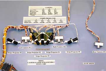
There were three imaging subsystems aboard the rover. Two broad-band
monochrome camera/laser systems were located on the forward part of
the rover, and a third camera was located on the aft part near the
APXS. The two front cameras, used in conjunction with laser stripe
projectors for hazard detection, provided images for stereoscopy and
measurements. The aft camera, which was rotated 90°, provided
spectral information while imaging the APXS target area, rover tracks,
and terrain. The 'cameras' were CCDs clocked out by the rover Central Processing Unit (CPU). The camera systems were capable of auto-exposure, block truncation coding (BTC) data compression, bad pixel/column handling, and image data packetizing. The major components of the camera systems are described in detail below. |
  |
| CCD array size | 484 (vertical) x 768 (horizontal) pixels |
 (Aft Camera Color Map) |
|---|---|---|
| Pixel size | 13.6 um (vertical) x 11.6 um (horizontal) | |
| Full well | 60,000 electrons (manufacturer claims 80,000) | |
| Output sensitivity | 10 uV/electron | |
| Dynamic range | > 60 dB | |
| Dark Noise | 40 electrons rms | |
| Dark Current | < 0.5 nA/cm2 | |
| Blooming suppression | > 300 X | |
| Maximum Data Rate | 14.3 MHz | |
| Image lag | negligible |
Aft Camera Specifications:
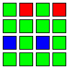
Same as the Front Camera specs, except that the CCD chip was engineered as a Color Filter Array. The pixels were arranged in a 'field-staggered 3G' color mosaic filter pattern. In each 4x4 pixel block, 12 were Green sensitive, 2 were Red sensitive and 2 were Blue sensitive. The blue pixels were sensitive to both blue and infrared wavelengths. Given that the camera optics blocked out much of the light in the blue part of the spectrum, the 'blue' pixels were essentially infrared pixels. (More information about the aft, color CCD is available in [DLUNA&FROSINI1992] and [PARULSKIETAL1992].) The pixel map for the color CCD is as follows:
| G | R | G | R |
| G | G | G | G |
| B | G | B | G |
| G | G | G | G |
This map repeats in both the row and column directions. This is the orientation of the pixel map for a rotated image, and thus will have to be rotated 90° to match the color map published by the manufacturer of the CCD (Eastman Kodak Company).
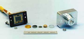
There were three elements that made up the optical subsystem: 1) camera window, 2) objective lens, and 3) field flattener lens. Their material makeup included optical grade sapphire and zinc selenide. This was significant in that the zinc selenide effectively blocked transmittance of most blue light. For a diagram of the optical elements, see document [SEPULVEDA1994].
| Camera window | Optical grade sapphire |
|---|---|
| Objective lens | Optical grade zinc selenide |
| Field Flattener lens | Optical grade zinc selenide |
General Camera Features:
The resolving power of the rover cameras contributed significantly to the technology experiments measuring grain sizes in surface material. The rover cameras were designed to be able to resolve fragments about 0.6 to 1.0 cm across at a nominal range of 0.65 m. Closer viewing of the surface near the wheels could reduce these sizes by four-tenths, and special situations (ie., close-up views of a rock 20 cm high) could reduce these values by as much as one-tenth.
| Lens focal length | 4 mm |
|---|---|
| Forward camera separation | 12.56 cm |
| Approximate height above surface | 26 cm |
Fields of View:
| Forward cross track | 127.5° |
|---|---|
| Forward along track | 94.5° |
| Aft cross track | 94.5° |
| Aft along track | 127.5° |
| Forward Boresight Angle | -22.5° |
| Aft Boresight Angle | -41.4° |
Average Spatial Resolution per Pixel:
Spatial resolution is the product of the distance of an object or surface from the camera and the camera resolution (in mrad/pixel). To calculate the average spatial resolutions, a camera resolution of 0.003153 mrad/pixel was used.
| Forward cross track | 0.166° (2.897 mrad) |
|---|---|
| Forward along track | 0.195° (3.409 mrad) |
| Aft cross track | 0.195° (3.409 mrad) |
| Aft along track | 0.166° (2.897 mrad) |
The filter on the front cameras was to have a peak transmittance of 97% at the central wavelength, which is defined as:
W = 860 nm + 30 nm / -30 nm
For every 4 x 4 block of pixels in the aft Color Filter Array, 12 were green, two were red, and two were infrared, allowing multispectral imaging of surface materials. Compared to the response for the red and green pixels, that of the infrared pixels was low. When exposure time was increased to improve the dynamic range of the infrared pixels, the impact was negative as light bled from the red and green pixels into the infrared pixels. As a result, the aft color camera was most useful in providing red and green color information. For a schematic diagram showing the relative spectral responses of the aft color camera, see Figure 5 in the [MATIJEVICETAL1997A].
| Forward Wavelength Sensitivity | 830 - 890 nm |
|---|---|
| Aft Wavelength Sensitivity | 500 - 900 nm |
Laser ranging:
Proximity scanning using the lasers was controlled by a table of camera/laser combinations. For each combination, a list of calibrated scan lines was stored. For each laser at each line, the nominal spot position, first-order scaling of pixel offset to height, and correction scale factors for pitch and roll were stored.
Image capture:
Image capture was executed by applying low-level functions to manage the acquisition, readout, and optionally, compression of the data. Valid image data were in rows 6 through 489 and columns 0 through 767; row 490 contained dark reference pixels. The data was packetized for telemetry, with enclosed identifiers describing the exposure (in milliseconds) and image region.
Auto exposure determination was indicated by an exposure time of zero. Given an image region, an overexposed image was taken and the brightest (saturated) pixel found. Then a geometric search of exposure times was performed, until an image was found with an average pixel value between 40% and 50% of saturation. Finally, exposure time was reduced by 25% as many times as necessary until no more than 1% of the pixels were within 5% of saturation. An exposure time of 1 indicated that the last computed auto exposure time was re-used. If no auto exposure had been performed since the last wakeup, a new auto exposure time was determined.
As part of the auto exposure, a shift factor was employed to manage the A/D conversion from 12 bits to 8 bits. Proper auto exposure for the front B&W cameras generally required a shift factor of 2, while the aft color camera used a shift factor of 1.
Compression:
Used optionally on front camera B&W images only, the block truncation coding (BTC) algorithm gave a fixed 4.9:1 compression ratio, helping to reduce the communication time without unduly sacrificing image quality. In pre-flight tests, a S/N ratio of 145:1 was achieved. Compression was performed on 16 column by 4 row blocks of image data. When the BTC compression was performed on aft camera images, a loss of color information resulted.
The data collected for the rover was then processed using a set of programs, collectively referred to as CCAL, to produce the CAHV camera models for each rover camera. A description of the CCAL software follows.
CCAL
These programs have been written for calibrating cameras for use in robotic machine vision. The programs were developed in the Robotics Vehicles Group (known by other names in years past) of Section 345 (formerly 347) at the Jet Propulsion Laboratory. The camera models are based on the linear models of Yakimovsky and Cunningham, were extended to include radial lens distortion by Gennery, and were further extended to include fish-eye lenses by Xiong and Gennery. The calibration measurement and reduction algorithms were designed by Gennery. For more information on the camera models, see the references below.
There are a number of programs for performing camera calibration. All of them assume that the cameras are mounted and/or aligned as needed prior to calibration, and that the user has some method of obtaining calibration images from the cameras stored into files. The file format used is a local format call PIC. This format is very simple. The first four bytes of the file are the integer number of rows in the image. The next four bytes are the integer number of columns in the image. Following these are the byte pixels in normal scan line order. While the nominal storage of the 4-byte integers is big-endian on all current systems (MSB first, LSB last), the software will recognize little-endian integers as well.
Most of the CCAL programs display graphical data by using the X windowing system, and therefore must be run under an X-based graphical user interface (GUI).
Calibration Overview
Camera calibration is broken into two major stages. The first is the collection of calibration data; the second is the reduction of those data to form camera models.
The calibration data is a collection of 3D-to-2D correspondence points. For each of a number of locations within the field of view of the camera, it is necessary to determine both its 3D world coordinate, and where it falls in the 2D image plane. The 3D locations of points must be non-coplanar in order to be able to solve for the camera-model parameters.
Two programs are provided to collect calibration data. One lets the user indicate with a mouse click where each of 2D points falls. The other does analysis of images showing a special calibration fixture in known locations. The output of both of these programs is a data file containing the 3D-to-2D correspondence data.
The next step involves using another program to reduce the data. Other programs may then be used to examine the resulting camera models.
Programs
The following is a brief overview of the calibration programs:
Ccal5d is used to make a manual collection of calibration
data. The user inputs 3D coordinates either interactively or from a
file and then specifies with a mouse click where in a displayed image
the corresponding 2D images points are located.
Ccaldots is used to analyze images of a special
calibration fixture in known locations. With minimal operator
initialization this program will determine 2D locations to sub-pixel
accuracy and match them up to the a priori 3D locations.
Ccaladj performs a least-squares fit of the calibration
data to the parameters of the camera models. It outputs the model
parameters along with covariance data. It can produce the old linear
perspective CAHV camera models, the newer CAHVOR models that include
terms for radial lens distortion, or the most recent CAHVORE models
that include a moving entrance pupil. Both perspective and fish-eye
lenses are handled in CAHVORE.
Ccalres graphically displays the residuals of the
calibration by examining the input data and comparing the input 2D
locations to the 2D locations computed with the camera model. The
user can scale the residuals for easy viewing.
Ccaldist displays the amount of distortion in a CAHVOR
camera model. It can render the display in a graphical form and in a
textual/numeric form. In the case of the numeric form, the user is
prompted for 2D image locations at which distortion information is
wanted.
MissionMars Pathfinder
TargetsPDS Welcome to the Planets: MarsPDS High Level Catalog: Mars
Instrument HostMars Pathfinder Rover
InstrumentMars Pathfinder Alpha Proton X-ray Spectrometer
|
Data Set DescriptionsAPXS Raw DataAPXS Oxide Abundances Rover Camera Raw Data Rover Camera Calibrated Images and Mosaics Rover Engineering Data ReferencesDLUNA&FROSINI1992GENNERY1991 GENNERY1993 GENNERY1994 GENNERYETAL1987 MATIJEVICETAL1997A PARULSKIETAL1992 SEPULVEDA1994 YAKIMOVSKY&CUNNI1978
|